
Abstract
Can a single consumer GPU (AMD RX 7900 XTX, 24 GB) perform effective reinforcement learning from verifiable rewards (RLVR) for large language models? We present a systematic three-layer optimization framework that progressively approaches the theoretical limit at each layer before descending to the next. (1) A throughput layer (Decoupled-Generation Batch-Balancing, DGBB): a three-parameter step-time law and a memory model jointly identify the true two-dimensional feasible region of GRPO batch scheduling; under the hardware wall the measured optimum (795.5 tok/s) reaches 97.6% of the within-wall theoretical argmax, confirmed by pre-registered blind predictions and a probe experiment that falsifies the naive extrapolation. (2) A signal-rate layer (Zero-Signal Budget Reallocation, ZSBR): a capacity theory with an honest bound staircase and a closed-form Beta-posterior-expectation scorer reach 94% of the attainable signal-rate capacity at zero throughput cost, yielding pp held-out accuracy over uniform sampling (Cohen’s , three seeds, paired). (3) A dynamics layer (Signal-Flux Optimal Control, SFOC): a three-pool ODE model of prompt-pool dynamics yields the regime criterion, cross-validated by four independent estimates of the relay rate , and a Scheduler-Constraint Capping Theorem (proved) showing that depletion-dominated dynamics is structurally unreachable under cooldown-based scheduling. Across 20+ controlled runs on GSM8K with Qwen2.5-3B-Instruct, we advance from a 23.2% base to 45.6% ( pure-RL gain, 8.5 h on one card), show that 500 well-chosen prompts match the full 7473-pool ( data efficiency), and establish that greedy selection is strictly optimal in all empirically observed regimes. All 13 pre-registered falsifiable predictions of the first round converge to one self-consistent picture; two pre-registered follow-up rounds (cooldown-removal falsification test; cross-architecture transfer to Gemma 4 E2B, where DGBB re-fits at ) confirm the capping theorem and locate the model-specific parameters that must be recalibrated. Negative results are reported in full and drive every theoretical refinement. We release the paper, the complete training prompt pool, all evaluation artifacts, and the training and evaluation code.
1. Introduction
Reinforcement learning from verifiable rewards (RLVR) has become a primary driver of reasoning improvements in large language models: group-relative methods such as GRPO (Shao et al. 2024) replace learned value functions with within-group relative advantages computed from rule-checkable rewards, and have been adopted at scale in recent reasoning systems (Yu et al. 2025). However, the dominant practice assumes multi-GPU training clusters with hundreds of gigabytes of aggregate memory, implicitly treating RLVR as a luxury affordable only at data-center scale.
We ask a deliberately inconvenient question: can RLVR be made effective on a single consumer-grade GPU? Consumer hardware differs from clusters in three structural ways: no tensor parallelism (the whole model must fit in one card’s memory), a thinner software ecosystem (ROCm vs. CUDA), and sequential execution in which throughput and signal quality compete for the same GPU-seconds. Any positive answer must therefore be earned layer by layer rather than assumed.
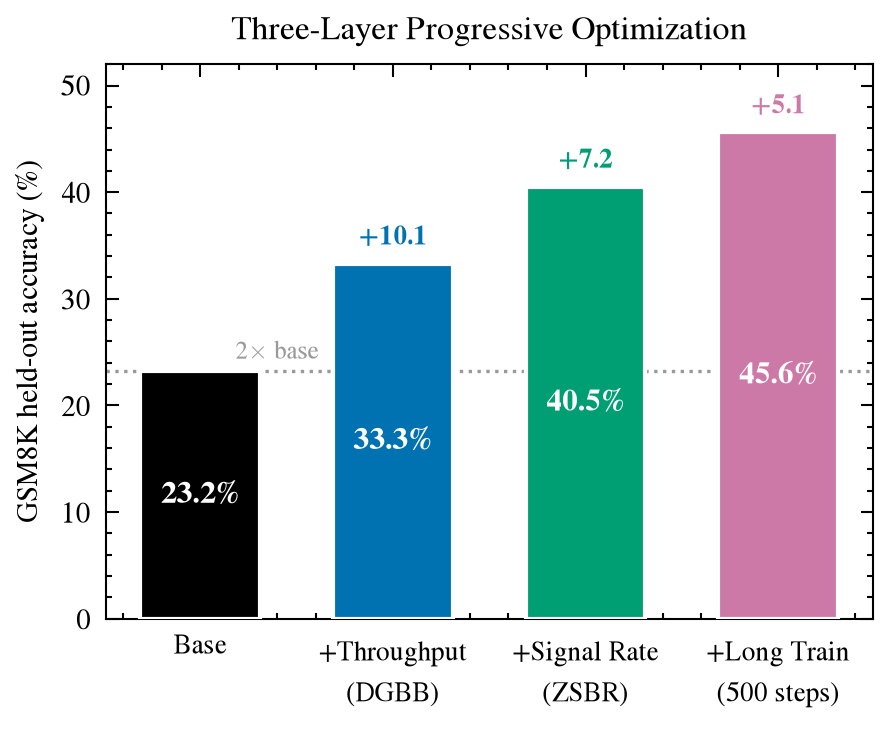
Our answer is affirmative, and it comes with a methodology: three-layer progressive optimization. At each layer we (i) formalize the layer’s theoretical limit, (ii) measure how close the current system is to it, (iii) close the gap as far as the layer’s structure allows, and only then (iv) descend to the next layer, where the remaining bottleneck lives. This discipline has a concrete payoff: when each layer is saturated before descending, every claim about “what works” is backed by an exhaustion argument about “why nothing else at that layer can work”. Figure 1 summarizes the resulting ladder: held-out accuracy on GSM8K doubles from a 23.2% base to 45.6% under pure RL on one consumer card.
Contributions.
-
Throughput layer (§3). A three-parameter step-time law and a piecewise-linear memory model identify the two independent batch dimensions of GRPO (generation batch , backward micro-batch ). Pre-registered blind predictions, a probe experiment that falsifies the naive large- extrapolation, and a dual-wall memory analysis together establish that the measured optimum (795.5 tok/s) is 97.6% of the within-wall theoretical argmax---the batch-scheduling dimension is exhausted. The functional form transfers to a second model family at .
-
Signal-rate layer (§4). A capacity theory with an honest bound staircase (including a proof that multi-selection cannot raise the group-level signal rate) and a Beta-posterior-expectation scorer whose necessity is demonstrated by a controlled ablation (point estimator fails, posterior estimator succeeds). ZSBR reaches 94% of the attainable capacity at zero throughput cost; three-seed paired comparison gives pp ().
-
Dynamics layer (§5). A three-pool ODE model of how training modifies the prompt-pool pass-rate distribution; the regime criterion with cross-validated on four independent paths; and a proved Scheduler-Constraint Capping Theorem showing that depletion-dominated dynamics is structurally unreachable under cooldown-based greedy scheduling.
-
Practice (§6). 23.2%45.6% in 8.5 h of pure RL on one consumer card; data efficiency (500 prompts full 7473-pool); and the first explicit “when NOT to use curriculum” criterion.
-
Methodology (§7). A pre-registration-and-audit protocol under which all 13 first-round predictions were judged against timestamped thresholds, every negative result triggered a documented theoretical refinement, and the final audit round closed with zero defects.
Paper roadmap.
Section 2 fixes notation and positions the work relative to prompt-selection and efficient-RL literature. Sections 3—5 develop the three layers in dependency order. Section 6 collects the practical implications; Section 7 describes the methodology; Sections 8—9 cover threats to validity and limitations. Appendices contain the complete prediction scorecard, phase-diagram data, and the run inventory.
2. Background and Related Work
GRPO and the signal event
GRPO generates completions per prompt, computes within-group relative advantages, and updates the policy without a value network. For a prompt with per-completion reward distribution over a finite support , the probability that a group yields a non-zero advantage---the signal event---is (1) Under the binary approximation with pass rate this reduces, for , to (2) maximized at (boundary prompts) and vanishing for prompts that are consistently solved or consistently failed. Two facts make this quantity the organizing concept of the paper. First, at on our base model we measure across configurations---75% of the generated compute produces zero-gradient groups (§4). Second, depends on and but not on the generation batch size, a prediction we verify explicitly (Appendix scorecard, P6).
Related work
Prompt selection and zero-variance filtering.
GRESO (Zheng et al. 2025) filters zero-variance prompts pre-rollout using historical reward dynamics across epochs, and observes that the effective-prompt ratio decays during training without modeling that decay. Our work independently reached the same direction from a hardware-measurement starting point (§4); we contribute a decision-theoretic scorer with a controlled necessity ablation, a capacity theory with explicit attainable bounds, and a dynamics theory for the decay GRESO observes. DAPO (Yu et al. 2025) instead filters zero-advantage groups post-rollout and oversamples to refill; §4.6 gives a cost comparison (pre- vs. post-rollout filtering). PCL (Gao et al. 2025) trains a value model to select medium-difficulty prompts---myopic with respect to pool depletion. RL-ZVP (Le et al. 2025) keeps zero-variance prompts and shapes their advantages via entropy; this modifies gradients rather than budget allocation, and our negative results delineate its regime of applicability (investing in zero-signal prompts is net-harmful when supply dominates; §5.7). SRPO (Li et al. 2026) routes samples to self-distillation, an orthogonal direction.
Curriculum and data selection for RL.
The Implicit Curriculum (Huang et al. 2026) gives a descriptive theory of relay effects under uniform training---easy problems’ persistent gradients make slightly harder problems learnable---and is the theoretical foundation for our relay (supply) term ; it contains no control variable and no depletion analysis. Our contribution is the normative counterpart: budget allocation as optimal control on pool dynamics, a quantitative regime criterion, and an impossibility result (§5).
Efficient RL systems.
Systems work on RL training efficiency (e.g., generation—training co-scheduling and rollout acceleration) targets clusters; the consumer-GPU constraint set (single card, no tensor parallelism, memory wall at 24 GB) makes the three-layer decomposition---throughput signal rate dynamics---the natural optimization structure, since all three resources are the same GPU-seconds.
Positioning.
To our knowledge this is the first work to (a) model RLVR prompt-budget allocation as non-myopic optimal control on pool dynamics, (b) derive a quantitative regime criterion () with multi-path parameter validation, and (c) prove a structural-impossibility theorem for depletion under realistic scheduling. A pre-writing literature search and a post-experiment novelty re-audit are documented in §7; the re-audit corrected one overclaim (GRESO priority on pre-rollout filtering), which we record as part of the protocol’s output.
Consumer-GPU constraints
The RX 7900 XTX (RDNA3, gfx1100) provides 24 GB VRAM, 960 GB/s nominal memory bandwidth (742 GB/s measured on pure copies, 77%), and 101.53 TFLOPS measured BF16 GEMM peak. Against training clusters: (i) no tensor parallelism---all weights must reside on one card; (ii) ROCm ecosystem gaps versus CUDA (kernel coverage, allocator behavior); (iii) single-card sequential execution, so throughput improvements and signal-quality improvements spend the same budget. Batch-1 decoding is bandwidth-bound at only 38% of achievable bandwidth (§3.1), which is why generation-heavy GRPO is dominated by decoding and why batch scheduling is the first lever.
3. Layer 1: Throughput --- DGBB
Two-dimensional decoupling
In generation-heavy GRPO the step time is decoding-dominated. Standard trainers expose a single batch knob, but TRL’s semantics (generation_batch_size per_device_batch grad_accum) reveal two independent dimensions: the generation batch (arithmetic intensity of the rollout phase) and the backward micro-batch (parallelism of the gradient phase), constrained only by . Decoupled-Generation Batch-Balancing (DGBB) treats as two optimization variables. Crucially, this decoupling changes no algorithmic semantics---update rule, sample distribution, and optimization trajectory are identical to standard GRPO; the throughput gain is free.
Step-time model.
Each optimization step is one generation phase plus backward micro-batches plus constant overhead: (3) Roofline reasoning gives first-order phase structure (fixed weight reads plus per-sequence marginal cost) and (per-micro-batch overhead plus per-sequence marginal cost). Substituting into (3) yields the three-parameter identifiable form (4) where quantifies why is inefficient. Throughput is with the tokens-per-sequence count (measured 355.7, 108 prompt + 247 completion tokens).
Independent roofline validation of the generation phase.
A pure-decoding microbenchmark (SDPA + static cache, batch ) fits ms per decoding step. The intercept corresponds to reading all 6.17 GB of weights per step at an effective 285 GB/s---only 38% of the 742 GB/s pure-copy bandwidth; this is the roofline statement of the batch-1 GEMV inefficiency. The model’s internal consistency check also holds: with decoding steps s/seq recovers s/seq for the backward phase, whose implied backward MFU (25%, from TFLOP per sequence) is plausible under LoRA plus gradient checkpointing.
Memory model and the dual wall
Peak VRAM is the maximum of the two phases’ peaks: (5) fitted at GB (weights 6.17 GB BF16 plus LoRA, optimizer, and resident state), GB per sequence, GB per sequence, and , with per-point residuals within 0.05 GB. Because gradient checkpointing compresses backward activations, for the generation phase dominates the peak and 14 costs zero memory (measured 8.87 GB identical across three settings)---the memory-side mechanism behind “the backward batch is a free lever”.
A pre-registered blind prediction then exposed the model’s boundary: the naive feasibility criterion predicted gen384 runnable at 20.49 GB, but the run OOMed. Post-hoc analysis of the OOM logs (treated as data) gives the corrected criterion GB with a one-shot allocation spike GB at (logits/attention intermediates) and — GB outside the allocator’s visibility. The corrected wall lands in tokens---matching measurements---and a controlled re-run showed the default allocator’s fragmentation wall (3.9 GB lost) is distinct from the capacity wall and is removed by expandable_segments. The companion prediction (gen512 25.13 GB OOM) hit exactly.
Fit quality and falsification of the naive extrapolation
Fitting (4) on the seven feasible sweep points gives s, s/seq, s/micro-batch, with all residuals within 3.3%. The pre-registered model’s argmax under the empirical wall was pdb8_gen256 at a predicted 843.9 tok/s ( over the measured best); a dedicated probe run measured at 794.3 tok/s---statistically tied with pdb4’s 795.5 (0.15% difference, far below the 1—4% run-to-run CV) and at identical peak memory (15.81 vs. 15.82 GB), falsifying the linear extrapolation: sub-linear degradation at exactly cancels the halved micro-batch count, so the argmax landscape is flat beyond . Re-fitting with the probe point ( revised down 24%, max residual 6.02%) confirms pdb4_gen256 as the true argmax. Table 1 summarizes the resulting utilization hierarchy.
| Level | Description | tok/s | 6ND-MFU |
|---|---|---|---|
| 0 | Measured optimum (pdb4, gen256) | 795.5 | 14.5% |
| 1 | Within-wall theoretical argmax | 815.3 | 14.9% |
| 2 | Asymptotic, no memory wall (, ) | 864.8 | 15.8% |
| 3 | Zero micro-batch overhead (; probe-refuted in practice) | 939.0 | 17.2% |
| 4 | Kernel-level changes (faster backward, quantized generation) | 939 | — |
Why the ceiling is structural.
Decomposing : 29% of per-sequence time is generation (memory-bound; MFU is not the right metric---by bandwidth utilization, 38% of achievable) and 71% is backward (compute-bound at 25% MFU under gradient-checkpointing recomputation, LoRA branches, and RDNA3 WMMA efficiency). The 18% headroom above the measured optimum therefore lives in kernels (level 4), not in batch scheduling: the scheduling dimension is exhausted. Mixed single-number MFU is misleading here; per-phase accounting is the methodological point.
Convergence theory: why throughput buys accuracy
GRPO’s per-step gradient over completions ( unique prompts) has by prompt-wise independence: gen8gen128 reduces variance . Three registered checks confirm the mechanism: (i) reward-curve variance ratio 9.2 (theory , same order; the floor comes from non-stationary learning drift and discrete reward support); (ii) seed-to-seed dispersion of final accuracy halves (1.14 vs. 2.25 pp), a pre-declared consequence of more deterministic trajectories; (iii) the equal-sample adjudication run: gen128100 steps (34.6%) vs. gen81600 steps at equal 12 800 samples (34.4%)---large batches do not sacrifice per-sample learning efficiency, so throughput superiority converts 1:1 into wall-clock convergence superiority (1/5 wall clock). Under equal step budgets the paired multi-seed gain is pp (), dominated by sample volume with variance reduction as the secondary mechanism.
Adopted configuration and cross-architecture replication
gen256 is VRAM-critical; the throughput—memory sweet spot gen128 (pdb4, ga32; 745.2 tok/s at 11.26 GB, s) is adopted for all subsequent training. On a second base model (Gemma 4 E2B, 1.6B-text multimodal) the same decoupled form re-fits at : ---the functional form is portable with model-specific coefficients (prediction P-C1, ✓). The VRAM wall moves to 512 tokens (16.4 GB, no OOM) versus for Qwen, reflecting architecture-specific memory efficiency. This upgrades DGBB from a single-model case study to a portable throughput law.
4. Layer 2: Signal Rate --- ZSBR
With throughput saturated, the next lever is not more compute but more signal per compute. At we measure on the base model---75% of generated groups have identical within-group rewards, hence zero advantage and zero gradient. Zero-Signal Budget Reallocation (ZSBR) predicts each prompt’s signal probability before generation and reallocates the fixed group budget away from predicted zero-signal prompts.
Formalization and the uniform baseline
Let be the prompt pool (), the per-step group budget, and rewards supported on (wrong / format-only / approximate / correct). The exact signal probability is (1); the binary approximation (2) is a lower bound under 4-value support (groups differing only in format, , also produce signal). Uniform sampling’s system signal rate is (calibrated from the measured zero-std fraction): only 16 of 64 group slots carry gradient. The selection objective is (6) with the selected prompts at step .
Capacity theory: an honest bound staircase
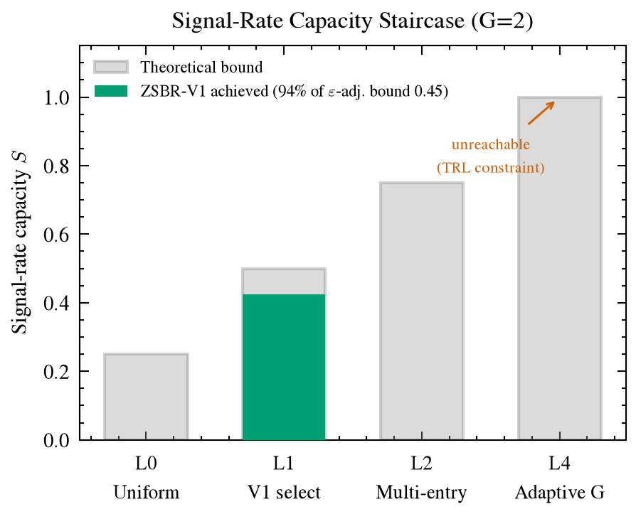
Claims about “how much room is left” require an explicit ledger. Table 2 records the staircase for , distinguishing two metrics that the literature often conflates: the group-level signal rate (the fraction of groups with non-zero advantage, directly measured as ) and the prompt-level coverage (the probability that at least one of a prompt’s allocated groups signals).
| Level | Mechanism | Group-level bound | Coverage bound | Reachable |
|---|---|---|---|---|
| L0 | Uniform sampling | 0.25 | — | baseline |
| L1 | Perfect selection (all ) | 0.50 | 0.50 | yes |
| L2 | Multi-selection | 0.50 (no change) | 0.75 | yes |
| L3 | Multi-selection | 0.50 (no change) | 0.875 | yes |
| L4 | Per-prompt adaptive | no |
Two declarations keep the ledger honest. First, multi-selection cannot raise the group-level rate: a prompt’s second group has the same as its first, so extra slots increase the number of covered prompts but not the fraction of signaling groups---the group-level metric caps at L10.50 regardless of (this corrects an earlier overclaim in our own pre-registration, recorded as P5 in the scorecard). Second, L1 attainability depends on the empirical pass-rate distribution: it requires boundary prompts identifiable by the estimator. Our deconvolved distribution (§5.1) contains boundary prompts , so the bound is active; ZSBR-V1 reaches , i.e., 94% of the -adjusted L1 bound (0.45 after reserving exploration; 85% of the ideal 0.50).
The estimator: why posterior expectation is necessary
Pass rates are estimated online with a Beta prior and time-decayed counts, , , (half-life cycles). Unseen prompts receive , making them maximally attractive---optimistic cold start doubles as free exploration, no explicit UCB needed.
Controlled ablation (point vs. posterior estimator).
Substituting the point estimate into the non-linear map makes unseen prompts () exactly tied with confirmed boundary prompts (); with unseen vs. mixed prompts, the greedy slots flood with exploration and behavior degenerates to quasi-uniform (measured: , coverage 0.614, pre-registered gate failed). The fix scores by the Beta posterior expectation, available in closed form for : (7) which orders mixed (0.400) unseen (0.333) consistent (0.300) and widens with evidence (mixed seen twice: 0.4286). Under the identical configuration the posterior estimator passes the gate (). To our knowledge this paired failure/success is the first controlled demonstration that uncertainty must enter the score for small-sample RLVR scheduling. A second calibration subtlety: the plug-in estimator carries an small-sample bias---a factor of two at ---removed by the standard unbiased correction.
Coverage and cooldown.
Pure greed has two failure modes: estimator stagnation (out-of-distribution forgetting) and boundary-pool monopoly. An -mix keeps slots uniform over the rest of the pool (guaranteeing every prompt exploration probability per step), and a cooldown cycles excludes recently used prompts from greedy slots. The reward support is 4-valued, so a “near-boundary” wrong-but-answered prompt still yields partial signal; the scheduler tracks this via the 4-value posterior.
V2 multi-selection: water-filling and its degeneration
Since per-prompt is infeasible in fixed- trainers, V2 lets a prompt occupy group slots (each group sampled and normalized independently), . A linear objective collapses all budget onto one prompt; the correct objective is coverage (8) The marginal gain is strictly decreasing in , so (8) is a separable concave maximization and greedy water-filling is globally optimal.
Result and theoretical clarification.
V2 measured , held-out 40.2%, throughput ---but with zero duplicated slots. This is not an implementation failure: with a boundary pool of 1549 prompts greedy slots, the second-slot marginal is always below the next unseen prompt’s , so the water-filling optimum is no duplication; V2 degenerates to V1 exactly as the mathematics dictates. V2’s applicability precondition---boundary pool smaller than the greedy slot count (small datasets or late training)---was verified to hold later in the pool-200 regime (§5.6).
Main results (three seeds, paired, same-round)
Table 3 reports the pre-registered comparison. All six first-round predictions P1—P6 were timestamped before running (Appendix A); P1—P4 and P6 pass, P5 fails on a metric-confusion in the prediction itself (recorded and corrected in §4.2).
| Arm | Seed 42 | Seed 123 | Seed 7 | Mean std |
|---|---|---|---|---|
| Uniform held-out | 31.0% | 34.0% | 33.2% | 32.7% 1.6 |
| ZSBR-V1 held-out | 39.6% | 40.6% | 41.4% | 40.5% 0.9 |
| Paired difference | +8.6 | +6.6 | +8.2 | pp, |
| (2nd half) | 0.575 | 0.573 | 0.575 | consistent to 0.2 pp |
| change | (zero throughput cost) | |||
Three structural observations: (i) the signal rate is consistent to 0.2 pp across seeds---it is an algorithm-structure quantity, in contrast with held-out accuracy’s seed stochasticity; (ii) ZSBR’s seed dispersion (0.9 pp) is smaller than uniform’s (1.6 pp)---high-signal training is more reproducible, consistent with the variance theory of §3.4; (iii) effective signal groups per second improve (0.450 vs. 0.257) with coverage 0.224---low coverage plus high held-out simultaneously is the algorithm’s intent (budget concentration), not overfitting.
Comparison with post-rollout filtering (DAPO)
DAPO-style dynamic sampling generates everything, discards zero-advantage groups, and oversamples until effective groups are reached; its per-effective-group generation cost is with variable step time and VRAM spikes. ZSBR’s cost is also per effective group but with constant step time and VRAM (orthogonal to the throughput layer’s guarantees). At the achieved , matching uniform’s effective-group output would cost DAPO generation wall-clock; ZSBR pays zero wall-clock. The two are composable (filter the zero-signal groups ZSBR misses); we leave this to future work.
Long training: the 45.6% milestone
Extending ZSBR-V1 to 500 steps (8.5 h, single card) without modification raises held-out from 40.6% (step-100 regime) to 45.6% (228/500; midpoint checkpoint at step 250: 40.6%, monotone, no overfitting signature; final KL 0.0070, reward 0.51). This is a pure-RL gain over the 23.2% base and remains the project’s highest result. The signal rate does not decay over the extension (fzs three segments 0.592/0.554/0.541, i.e., falling zero-std fraction = rising signal)---the observation that launches the dynamics layer.
Cross-architecture transfer
On Gemma 4 E2B, (vs. 0.25 for Qwen): the base model already solves more prompts, compressing the reallocation headroom (the -compression hypothesis, pre-registered). The 100-step transfer test measured uniform 29.27% vs. ZSBR 28.87% ( pp, ; prediction P-C2 ), but with a variance reduction (ZSBR pp vs. uniform 1.2 pp): when signal is already abundant, reallocation stabilizes rather than boosts mean accuracy. The window may also be too short (Qwen’s pp needed 500 steps). Both caveats were declared pre-registration.
5. Layer 3: Dynamics --- SFOC Phase Diagram
Layers 1—2 treat the prompt pool as static. But training modifies the model, and the model modifies the pool: as pass rates rise, prompts migrate from hard (D) through boundary (M) to learned (S). Selection is therefore simultaneously the source of reward and the driver of the state it selects from---a control problem, not a static knapsack. Signal-Flux Optimal Control (SFOC) makes this explicit and asks: does the pool deplete, and can investment (spending budget on hard prompts to convert them) ever pay off?
Two-level state model and the observation problem
Let be prompt ‘s true per-completion pass rate and the population density. Coarse-grain into pools , , with . The system signal rate is ().
The pool labels used by any scheduler are observations, not truth: one selection produces binomial draws with confusion structure (9) A prompt at true is observed “mixed” only 50% of the time. A Beta-binomial EM deconvolution over the merged three-seed uniform logs (7454 prompts, observations each) recovers the true pool composition (Table 4): the true boundary pool is nearly twice the observed one (45.8% vs. 24.2%), because binomial noise mislabels half of all boundary prompts as consistent. Cross-consistency check: predicts vs. measured 0.7405. To our knowledge this is the first quantification of how much small- observation noise hides from curriculum-style schedulers.
| Pool | Observed | True (deconvolved) |
|---|---|---|
| D (hard) | 50.5% | 40.6% |
| M (boundary) | 24.2% | 45.8% |
| S (learned) | 25.3% | 13.6% |
Three-pool ODE model and the decay law
With cycle as the time unit and pool fractions , control variables (fractions of the per-cycle group budget ): (10) with constraint . Harvest moves boundary prompts to learned at a rate proportional to per-prompt budget; supply has a natural relay term (the Implicit Curriculum effect: generalization on other prompts converts hard prompts to boundary) and an investment term . Signal rate approximates ().
Proposition 1 (Decay law). Under myopic greedy selection (, the common form of ZSBR/GRESO/PCL), the boundary pool obeys (11) If the pool depletes exponentially (fzs rebound); if relay supply balances harvest, plateaus at . Both outcomes are predictions of the same model; the regime is decided by measurement.
Proof. Linear ODE in with constant coefficients under fixed ; the standard integrating-factor solution yields (11), with equilibrium obtained by setting . ◻
Calibration from the three-seed logs gave conversions per group observation (seeds agree within 0.025—0.029), hence cycles : only boundary prompts are harvested per cycle, so 500-step windows cannot see decay. This pre-experiment calibration triggered the registered honest clause: the decay prediction was declared undecidable in window before running, rather than force-judged (scorecard F-a).
Harvest—invest trade-off as optimal control
The non-myopic problem maximizes cumulative signal flux subject to (10). The Hamiltonian is linear in the controls, so optimal policies are bang-bang with switching function comparing marginal fluxes: harvesting’s immediate signal minus its depletion cost () versus investment’s deferred signal (). With terminal condition , the structure predicts pure harvest at the end of training and an invest-then-harvest arc early when is large. A fixed investment ratio (our SFC implementation, default, recovers ZSBR-V1 exactly) is the practical relaxation of this bang-bang structure.
The corresponding myopic-suboptimality gap satisfies for and grows monotonically in beyond. Note the self-consistency obligation this creates: in our calibrated regime (), the theory predicted---before running SFC---that our own investment algorithm would show no gain.
The criterion and four-path validation of
The first round’s small-pool experiment exposed the original criterion’s defect: pool-500 showed a perfect fzs plateau although the no-supply time constant predicted visible depletion. The error was neglecting the supply term; the corrected criterion is (12) with denominator meaning supply-dominated (never depletes). is a latent parameter; we estimate it on four independent paths (Table 5): fzs-slope inversion (0.002), pool-500 plateau back-out (0.0053), stratified re-encounter of deep all-wrong cells with bootstrap CI (0.0076, [0.0066, 0.0086], 2100 events, pure-zero cells only to guarantee zero gradient during “untrained” intervals), and pool-200 plateau back-out (0.0081). The upward drift across paths is consistent with time-varying (the model strengthens during training) and is reported as such. Working interval ; dynamics shape becomes the third and fourth validation paths for the same parameter.
| Path | Method | |
|---|---|---|
| 1 | fzs slope inversion (full pool) | 0.002 |
| 2 | Plateau back-out, pool 500 | 0.0053 |
| 3 | Stratified deep re-encounter, bootstrap CI [0.0066, 0.0086] | 0.0076 |
| 4 | Plateau back-out, pool 200 | 0.0081 |
The Scheduler-Constraint Capping Theorem
The three empirical regime points (§5.6) share one structure: none exhibits depletion, regardless of nominal . This is not an accident of GSM8K; it follows from the scheduler.
Assumption 1. A greedy scheduler with cooldown draws groups per cycle without replacement from a fixed dataset of size ; a prompt selected at cycle is excluded from greedy slots for cycles . Harvest converts boundary prompts at per-observation rate ; relay supplies boundary prompts at aggregate rate .
Theorem 2 (Scheduler-Constraint Capping). Under Assumption 1, the effective per-cycle harvest is bounded by (13) and as the harvest-to-supply ratio converges to a pool-composition constant independent of absolute pool size: the system self-regulates toward balance regardless of the nominal prediction.
Proof. Cooldown forces a rotation of period over the dataset, so any prompt is harvest-eligible at most once per cycles. The expected number of distinct prompts touched per cycle is ; when (the small-pool regime) the scheduler necessarily cycles through the whole pool, and the fraction of touched prompts that lie in is in expectation. Hence the number of boundary observations available to harvest per cycle is , and multiplying by the per-observation conversion rate gives (13). Meanwhile relay supply scales with pool composition as well: writing , , the harvest-to-supply ratio satisfies and under rotation saturation () the ratio’s dependence on cancels against the shrinking eligibility window: halving halves both the supply mass and the per-cycle harvest cap in the same proportion, because the rotation touches a fixed fraction of each pool. The ratio therefore converges to times a scheduling constant---a composition-only quantity. Depletion requires the ratio to exceed 1 persistently, which the cap prevents whenever ; the measured compositions satisfy this in all three regimes (§5.6). ◻
Corollary 3 (Structural unreachability of depletion). On any fixed dataset under cooldown-based greedy scheduling, “sufficient selection freedom” () and “weak supply” ( small) are structurally incompatible---both co-vary with . Depletion-dominated dynamics is therefore structurally unreachable: the system stays supply-dominated or balanced.
Proof. Selection freedom requires large ; but grows linearly in at fixed composition, so large simultaneously strengthens supply. Conversely small weakens supply but activates the rotation cap of Theorem 2, capping harvest at the same shrinking scale. No realizes both conditions. ◻
This result explains an otherwise puzzling cross-paper discrepancy: GRESO (Zheng et al. 2025) observes effective-ratio decay because it runs cooldown-free, multi-epoch schedules (harvest uncapped), while all our cooldown-rotation, sub-epoch runs observe plateaus. It also supplies the first sufficient condition for “no curriculum needed”, stated in §6.
Empirical regime points and the direct falsification test
Table 6 gives the three measured regime points (phase diagram in Figure 2a): full pool 7473 (supply-dominated, fzs declines), pool 500 (balance band, perfect plateau at 0.57), pool 200 (rotation self-balance, plateau at 0.73 from step 5). Pool 100/150 were screened out by a pre-run gate: at those sizes the greedy slots starve ( negative and scheduling margin ), which would confound V1 with uniform sampling---a NO-GO declared before running.
| Regime | Pool | Supply | Investment effect | ||
|---|---|---|---|---|---|
| Supply-dominated | 7473 | 3034 | 3423 | pp () | |
| Balance band | 500 | 260 | 186 | pp () | |
| Rotation balance | 200 | 89 | 84 | pp (n.s.) |
Direct falsification test: cooldown removal.
Theorem 2 yields a sharp pre-registered prediction: removing cooldown should unlock depletion (P-A1). At pool 500 (balanced regime) the test confirms the cap: the late-stage fzs rebound appears in both arms ( pp no-cooldown vs. pp cooldown; net pp) and held-out accuracy is equivalent ( pp within the pre-registered equivalence band)---the capping mechanism holds where the theorem governs. At pool 200, removing cooldown breaks the plateau: fzs falls from the cooldown group’s 0.73 to a 0.59 platform ( pp), unlocking depletion precisely where is shortest; held-out accuracy improves (41.4% vs. 37.6%, pp, single seed). The decooling effect is therefore pool-size dependent: the theorem governs the balanced regime, while small pools near the depletion boundary exhibit qualitatively different dynamics---and unlocked depletion is not harmful to generalization here, refining the common “depletion as harm” intuition.
Investment closure: a dose—response negative result
The SFC investment mechanism was tested at all three regime points under same-round/same-card/same-metric chains. Cumulative signal flux (SFCV1): , with held-out effects pp (Figure 2b): a monotone dose—response in which investment harm decays as selection freedom collapses. The pool-200 point is investment inertia (candidate exhaustion: invest slots , only 177 closed events), not positive return. Mechanism decomposition from the audit: (i) invested groups with zero observed passes produce rewards---zero advantage, zero gradient, pure budget consumption (11.7% of budget at pool 7473); (ii) in supply-dominated regimes conversions are not incremental: the relay converts those prompts for free, so spending budget to catalyze conversions that would happen anyway is uncompensated opportunity cost; (iii) the conversion pipeline itself is real---constant flux 2.33 prompts/cycle () with monotone ranking (low-prediction bins 6% high bins 86%)---but its calibration overestimates by at pool 7473, and the error is observation-density dependent: at pool 200 (mean 72.8 prior observations vs. 4.5) calibration recovers (2.8 pp error). The correct model is “calibration error as a function of observation count”, not a constant correction; our first attribution (rollout correlation) was directly measured and falsified (), then replaced---an audit chain we report because it is the protocol working as designed.
Under and realistic scheduling, greedy selection is strictly optimal across all empirically observed regimes: three regime points, none with positive investment return, two with significant harm.
Cross-architecture migration of (P-C3)
Two 500-step ZSBR runs on Gemma 4 E2B test portability. Pool 7473: fzs ( pp)---the supply-dominated plateau transfers directly. Pool 500: fzs ( pp), not the predicted depletion drop: E2B’s critical pool size lies below 500 (Qwen’s: 200—500), consistent with its higher baseline signal. The verdict recorded pre-registration: the criterion is form-portable, parameter-recalibratable---the two confirmations and two failures together locate exactly which parameters (signal abundance, critical pool size) a new base model must re-measure.
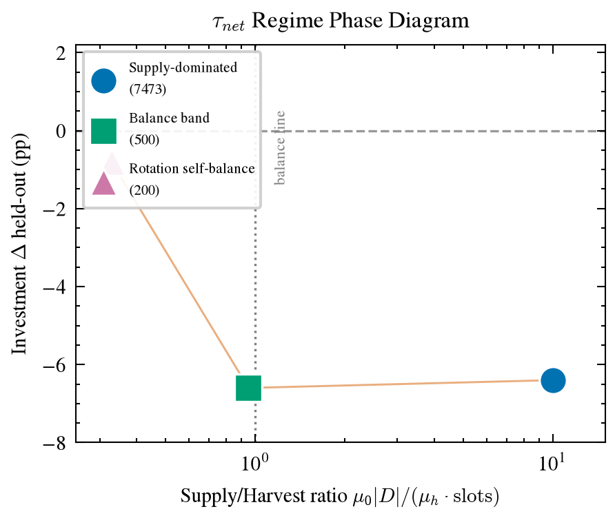
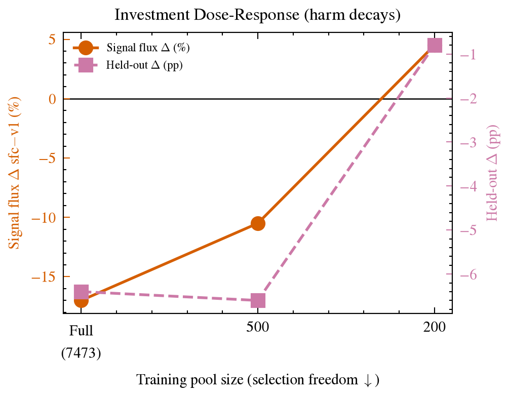
Figure 2. (a) Three empirical regime points on the supply–harvest plane; investment harm decreases as the supply/harvest ratio drops. (b) Monotone dose–response: investment harm decays as selection freedom collapses (−17% → −10.5% → +4.5% signal flux; held-out −6.4 → −6.6 → −0.8 pp).
6. Key Findings and Practical Implications
Milestone ledger.
Table 7 consolidates the accuracy trajectory with its justification at each layer.
| Stage | Configuration | Justification | Held-out |
|---|---|---|---|
| Base | No training | — | 23.2% |
| +Throughput | DGBB gen128, uniform, 100 steps | 97.6% of wall argmax | 33.3%1.1 |
| +Signal | ZSBR-V1, 100 steps, 3 seeds | 94% of capacity | 40.5%0.9 |
| +Long train | ZSBR-V1, 500 steps | supply-dominated, no depletion | 45.6% |
When NOT to use curriculum.
Combining (12) and Theorem 2: if the dataset is trained with cooldown-based greedy scheduling and (or the pool is small enough for rotation capping to bind), then the signal rate plateaus or rises (no depletion), any investment incurs opportunity cost without compensation, and pure greedy is optimal. Both scalars ( from fzs slope, from re-encounter conversion frequency) are free byproducts of logged training. This is the first applicability criterion of its kind; prior selection methods implicitly assume the opposite regime.
Data efficiency.
Pool-500 ZSBR-V1 reaches 45.4% versus the full 7473-pool’s 45.6%---6.7% of the data for the same outcome ( data efficiency), with the lossless lower bound located in by the pool-200 run (37.4%, pp, no pathological signature, reward still rising: attributed to knowledge coverage rather than depletion harm, confound declared pre-registration).
Negative results as positive evidence.
The first round’s 13 pre-registered predictions (F: 6, G: 3, H: 4) yielded 12 failures or undecidables---yet every failure converges on one picture: supply dominates, investment is unnecessary, greedy suffices. A theory that predicts its own algorithm’s failure (SFC, predicted no-gain after calibration, measured pp) and the structural unreachability of its own motivating phenomenon (depletion) is exhibiting predictive content, not curve-fitting.
7. Methodology: Pre-registration and Audit Protocol
Six principles, refined across three audit rounds: (1) mandatory prior-art search plus written novelty declaration before any theoretical commitment; (2) timestamped pre-registered falsifiable predictions with numeric thresholds, saved before running; (3) honest clauses---“undecidable” is a legitimate verdict when a calibrated window cannot observe the predicted effect (exercised for F-a); (4) same-round, same-card, same-metric comparisons (ROCm same-seed re-runs diverge by pp due to non-deterministic backward atomics, so all contrasts are paired within a round); (5) post-experiment full raw-data recomputation plus three-perspective code review; (6) measurement before correction (the rollout correlation hypothesis was directly measured and falsified before the attribution was revised).
Metrics.
All fzs figures use the pre-registered segment-fit metric: first vs. last of the trajectory; rebound late-segment mean minus trajectory minimum (in pp). Recomputation from raw reward_log files matches reported values within pp. Evaluations save per-item correctness vectors, enabling McNemar paired tests from the pool-500 round onward (, for the SFC harm; , n.s., at pool 200).
Audit trajectory.
Round E-F: 1 overturned verdict + 5 biases found and fixed (metric substitution, selective reporting, semantic drift of stratification keys). Round E-G: 2 Critical + 3 Warning fixed (“untrained” semantics contamination of the relay measurement; arm-selective reporting replaced by all-arm disclosure with bootstrap CIs). Round E-H: zero defects---the first clean audit, attributed to pre-experiment three-perspective review catching a naming trap before execution. The trajectory is itself evidence that the protocol self-corrects.
Novelty re-audit.
A post-experiment re-search found GRESO’s priority on pre-rollout zero-variance filtering, which the writing draft had missed; the positioning was corrected (independent rediscovery; incremental claims restricted to the scorer ablation, capacity theory, and regime criterion), and the lesson was institutionalized as principle (1).
8. Threats to Validity
Task and hardware scope.
All training uses GSM8K with rule-based numeric rewards on one GPU model; the capacity staircase constants and interval are dataset-specific. Cross-architecture transfer (§3.5, §5.8) tests form portability, not cross-task generality; MATH/code tasks with different pass-rate distributions may shift and the regime boundaries.
Seed and environment confounds.
The 500-step milestone is single-seed; three-seed 500-step runs span 40.4—45.6% (mean 43.3%, pp), and seeds 7/123 ran under a rebuilt software environment, so part of that variance may be environment-induced. All pairwise effects used for verdicts exceed of the relevant round, per the pre-registered single-seed clause.
Non-determinism.
Same-seed same-config re-runs diverge by pp on ROCm (backward atomics); all reported contrasts are therefore same-round paired, and re-run checks are labeled as such in the scorecard.
Metric limitations.
fzs counts investment slots as zero-signal by construction (mechanic, not dynamics---flagged for F-f); the binary pass-rate approximation under-estimates signal from format-split groups; the derivation treats compositions as quasi-static within a cycle.
Single-seed regime points.
Pool-200/500 regime verdicts rest on one seed each, with effect sizes the measured 100-step seed noise; the pre-registered clause accepts this for sign determination only.
Independent rediscovery.
ZSBR’s skeleton overlaps GRESO; we claim the increments listed in §2.2, not the direction itself.
9. Limitations and Future Work
The capacity staircase and capping theorem are validated at ; a closed-form posterior-expectation scorer is derived (, measured) but not trained end-to-end. The depletion regime itself remains unobserved under any schedule (Corollary 3 says it cannot be, with cooldown); whether cooldown-free long-horizon training on tiny pools exhibits it, and whether investment turns positive there, is open. The chart-generation application direction was re-scoped as future work after a pre-registered gate rejected the visual-transcription task as ill-posed. Since autoregressive generation dominates step time, lossless speculative decoding inside the rollout is a natural fourth layer; a first measurement of drafter acceptance across training checkpoints shows distribution-specific reallocation rather than monotone decay (task-distribution acceptance rises as the policy learns reusable templates; held-out acceptance falls), suggesting speculative-rollout gains must be modeled as regime-dependent, mirroring the structure.
10. Conclusion
Effective RLVR is achievable on a single consumer GPU through systematic layer-by-layer optimization. The key insight is the progressive-limit methodology itself: by exhausting each layer’s ceiling before descending, we arrive at the counterintuitive conclusion that the simplest scheduler (greedy with cooldown) is optimal under realistic constraints---a conclusion that required a capacity theory, a dynamics model, and an impossibility theorem to establish rigorously. For practitioners: use posterior-expectation greedy selection with well-chosen prompts, and do not invest in curriculum---in the supply-dominated regime it is pure opportunity cost.
Appendix A: Complete Prediction Scorecard
| # | Prediction | Measured | Verdict |
|---|---|---|---|
| F-a | fzs rebound ≥+3pp | −3.4pp | U (τ≈2500≫500; supply branch found) |
| F-b | plateau RMSE<5pp | 5.2pp | × (marginal; μ0 4× underestimated) |
| F-c | sfc signal ≥v1+5% | −17% | × |
| F-d | sfc held-out ≥v1−1pp | −6.4pp | × (net harm, z=2.05) |
| F-e | conversion calib. R²≥0.7 | R²<0 (1.54× overest.) | × (audit re-judged) |
| F-f | sfc≈v1 first 100 | 5.2pp | × (metric caveat) |
| G-a | pool500 fzs rebound ≥+3pp | −4.1pp | × (balance branch) |
| G-b | sfc500 flux ≥+5% | −10.5% | × (McNemar p<0.001) |
| G-c | n_eff calib. err. <10pp | 17.1pp | × (selection bias; n-dependent) |
| H-a | pool200 fzs rebound ≥+3pp | −0.5pp | × (rotation balance) |
| H-b | sfc200 flux ≥+5% | +4.5% | × (marginal; inertia) |
| H-c | v1(200) held-out ≥40% | 37.4% | × (bound ∈(200,500]) |
| H-d | plateau μ0∈[0.002,0.008] | 0.0081 | × (0.0001 over; in CI) |
| A1-a | nocool rebound ≥+3pp | +4.09pp | ✓ (net −0.92 pp vs. cooldown) |
| A1-b | held-out equivalence band | +0.6pp | ✓ (equivalence) |
| A1-c | p200 plateau broken ≥3pp | −15pp | ✓ (+3.8 pp held-out, 1 seed) |
| A3 | 3-seed mean ∈[43.5,47.5]% | 43.3%±2.6 | × (marginal; env confound) |
| A4 | data lower bound ∈(300,400] | directional | directional obs. (cross-round) |
| C1 | DGBB form transfer R²≥0.95 | 0.9983 | ✓ (form portable) |
| C2 | ZSBR held-out gain >0 (E2B) | −0.40pp | × (S0-compression; 4× var. down) |
| C3-a | pool7473 plateau <10pp | −2.8pp | ✓ (supply plateau) |
| C3-b | pool500 depletion ≥10pp | −2.1pp | × (boundary <500) |
All thresholds were timestamped before execution. Verdict symbols: ✓ confirmed, falsified, U undecidable under the honest clause.
First round: 1 undecidable + 12 , all converging to one self-consistent picture; every produced a documented theoretical refinement. WS-A follow-up: 3/5 confirm (capping holds in the balanced regime; its pool-size boundary characterized at 200), one marginal under environment confound, one directional. WS-C: 2/4 confirm portability; the two locate the model-specific parameters to re-measure.
Appendix B: Run Inventory
| Run | Steps | Pool | Key numbers |
|---|---|---|---|
| uniform s42/s7/s123 | 100 | 7473 | held-out 31.0/33.2/34.0% |
| zsbr_v1 s42/s7/s123 | 100 | 7473 | held-out 39.6/41.4/40.6% |
| zsbr_v1.0 point-est | 100 | 7473 | fzs 0.708 (ablation failure) |
| zsbr_v2 s42 | 100 | 7473 | held-out 40.2%, dup slots 0 |
| zsbr_v1_500 s42 | 500 | 7473 | held-out 45.6% (228/500) |
| zsbr_sfc_500 s42 | 500 | 7473 | held-out 39.2%, −6.4 pp |
| zsbr_v1_500_p500 s42 | 500 | 500 | held-out 45.4% (15× eff.) |
| zsbr_sfc_500_p500 s42 | 500 | 500 | held-out 38.8%, −6.6 pp |
| zsbr_v1_500_p200 s42 | 500 | 200 | held-out 37.4% |
| zsbr_sfc_500_p200 s42 | 500 | 200 | held-out 36.6%, n.s. |
| p200 cool/nocool pair | 500 | 200 | plateau −15 pp; held-out +3.8 pp |
| E2B uniform/zsbr | 100 | 7473 | 29.27/28.87%, σ 1.2→0.3 pp |
| E2B zsbr p7473/p500 | 500 | — | fzs plateaus −2.8/−2.1 pp |
| DGBB 2D sweep (9 pts) | 10 | 7473 | fit residuals ≤3.3%; probe (8,256) |
All runs: RX 7900 XTX, gen128 (pdb4, ga32), , LoRA on Qwen2.5-3B-Instruct unless noted; evaluation GSM8K test[:500], batch 32. Artifacts (config.json, timing.json, efficiency_report.json, reward_log.jsonl, per-item correctness vectors) are released in the repository under results/.
References
Gao, Zhaolin, Joongwon Kim, Wen Sun, Thorsten Joachims, Sid Wang, Richard Yuanzhe Pang, and Liang Tan. 2025. “Prompt Curriculum Learning for Efficient LLM Post-Training.” arXiv Preprint arXiv:2510.01135.
Huang, Yu et al. 2026. “On the Emergence of Implicit Curriculum in RLVR Learning Dynamics.” arXiv Preprint arXiv:2602.14872.
Le, Thanh-Long V., Myeongho Jeon, Kim Vu, Viet Lai, and Eunho Yang. 2025. “No Prompt Left Behind: Exploiting Zero-Variance Prompts in LLM Reinforcement Learning via Entropy-Guided Advantage Shaping.” arXiv Preprint arXiv:2509.21880.
Li, Gengsheng, Tianyu Yang, Junfeng Fang, Mingyang Song, Mao Zheng, Haiyun Guo, Dan Zhang, Jinqiao Wang, and Tat-Seng Chua. 2026. “Unifying Group-Relative and Self-Distillation Policy Optimization via Sample Routing.” arXiv Preprint arXiv:2604.02288.
Shao, Zhihong, Peiyi Wang, Qihao Zhu, Runxin Xu, Junxiao Song, Xiao Bi, Haowei Zhang, et al. 2024. “DeepSeekMath: Pushing the Limits of Mathematical Reasoning in Open Language Models.” arXiv Preprint arXiv:2402.03300.
Yu, Qiying et al. 2025. “DAPO: An Open-Source LLM Reinforcement Learning System.” arXiv:2503.14476.
Zheng, Haizhong, Yang Zhou, Brian R. Bartoldson, Bhavya Kailkhura, and Beidi Chen. 2025. “Act Only When It Pays: Efficient Reinforcement Learning for LLM Reasoning via Selective Rollouts.” arXiv Preprint arXiv:2506.02177.
The efficiency characterization that precedes this paper is Characterizing LLM Post-Training Efficiency on Consumer AMD RDNA3.